Something I’ve been working on quietly for a while is now ready. Four reference booklets, one each on equalizers, compressors, reverbs, and saturation. These are tools I reach for every day on the mix stage.
If you’ve been reading this blog over the past year, you’ve seen the posts on these same four topics. The booklets are those posts taken much further. I have a nod to the history and a lot of the working ideas that come from my mix experience. Each booklet is around 120 to 140 pages, organized with information the way I would have wanted to read them when I was learning.
What I tried to do with these is something I haven’t really seen done elsewhere. We start at the fundamentals, the actual physics of what is happening. Then into the workings, what the controls really do when you turn them. Then into the analog circuits, because that is where the character of these tools comes from, and knowing that is a blessing in disguise. And then into the plugins, how those same circuits get modelled in the software we reach for every day. The whole journey, end to end. The maths shows up only where it actually changes a decision you would make.
These are written for working mixers and serious students. Intuitive rather than academic. You can keep them open on the desk while you mix.
Each booklet is $15. The complete set of four is $40.
Every sound we hear has some kind of an audio signature to it. A boom microphone pointed at an actor on a wooden floor captures not just their voice but also the room’s resonant modes, the rumble of an air handler three floors up, the particular coloration of the mic capsule, and the way the voice bounces off the nearest hard surface before hitting the diaphragm. You see, even in a perfectly designed recording environment, no microphone is perfectly flat across the human hearing range, no source sounds the same from one position as another, and no recording chain from capsule to converter is neutral. In fact, the equalizer exists because sound, when left to its own, rarely arrives at the listener’s ears in the shape the recording demands.
The word Equalizer (EQ) itself actually tells an interesting story. It comes from early telephone engineering, where signals traveling down copper wire arrived at the far end with their high frequencies majorly reduced. It was because the resistance of long cables combined with the cable’s capacitance caused that. So, engineers built circuits to put back what was lost and to make the received spectrum equal to what was transmitted. Basically, the job was correction. It was processing the signal received, to be equal to the signal sent. That corrective function was the Equalizing part and it stayed. It expanded as audio recording became an art form and later became tone shaping.
The first audio equalizers appeared in the late 1920s and early 1930s, mostly as simple passive networks built into console channel strips. By the 1950s, two innovations changed what was possible. Peter Baxandall published an elegant active bass and treble tone circuit in Wireless World magazine in 1952. The design was freely given to the industry and has since appeared in virtually every hi-fi amplifier and mixing console on the planet. At almost exactly the same moment in New Jersey, Gene Shenk and Ollie Summerlin were hand-building the Pultec EQP-1 at their company Pulse Techniques Inc., which they had founded in 1953. The Pultec was something genuinely new. It was a passive program equalizer with a tube makeup amplifier, giving us a tool with broad, musical curves that could shape the spectrum without surgical precision but with exceptional audio grace.
The parametric equalizer arrived in 1972. George Massenburg, working at ITI Audio Products in Baltimore, presented a paper at the 42nd AES Convention in Los Angeles titled “Parametric Equalization.” His design used all-active RC circuitry to achieve continuous variable control over three independent parameters for each band: frequency, amplitude, and shape. That paper is available as Open Access from the AES E-Library, and it remains the foundation on which virtually every modern equalizer is built.
From here, the world of EQ expanded into such beautiful domains and technologies, that it became an inevitable tool and a creative add-on for all of us. But first, let’s get to understand how an EQ works and begin by looking at filters.
2 How a Filter Works
An equalizer is basically a collection of filters and a filter is a circuit or algorithm that passes certain frequencies and attenuates others. Everything else is a variation on this concept. To understand the EQ, you need to know not just what a filter does to audio but how it does it physically.
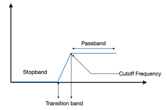
Now, there are four terms that we need to know when it comes to filters.
The passband is the range of frequencies the filter is supposed to pass without significantly affecting them. I say significantly because you’ll see that some filters do affect them. In a high-pass filter set to 100 Hz, the passband is everything above 100 Hz. In an ideal filter, every frequency in the passband would pass through at exactly the same level, completely unaffected. In reality, the passband is never perfectly flat. There is always some small variation. How much variation is allowed, and what shape that variation takes, is one of the key differences between filter families which we will see later.
The stopband is the range of frequencies the filter is supposed to block. So, in a high-pass filter set to 100 Hz, the stopband is everything well below 100 Hz. Again, in an ideal filter, the stopband would have infinite attenuation and nothing would get through. In a real filter, attenuation in the stopband is always finite. How deep that attenuation goes, and how evenly it is distributed across the stopband, is another key difference between filter families.
The transition band is the region between the passband and the stopband. It is where the filter is in the process of going from passing to blocking. Kind of like the part under the slope. No real filter has an infinitely sharp edge. There is always a frequency range where the filter is partially attenuating the signal but has not yet reached full stopband attenuation. The width of this transition band, and the shape of the attenuation curve within it, is the most important practical difference between filter families. A narrow transition band means the filter goes from passing to blocking quickly, over a short frequency range. The slope is steep. A wide transition band means the filter eases gradually from passing to blocking over a larger frequency range.
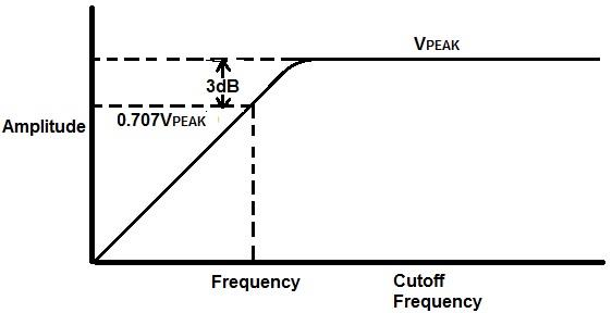
The cutoff frequency is the boundary point between the passband and the transition band. By convention, it is defined as the frequency at which the filter has attenuated the signal by 3 dB relative to the passband level. A loss of 3 dB also means that the power is reduced by half. Three decibels is roughly the point where most listeners begin to notice a level difference. So the cutoff frequency is the point where the filter has made its first clearly noticeable reduction to the signal. This 3 dB definition is a convention, not a physical law. Some filter families define their cutoff differently, which is one reason why comparing filters from different families at the same nominal cutoff setting can occasionally be misleading.
2.1 Analog Filters
Low Pass Filter
Low Pass Filter
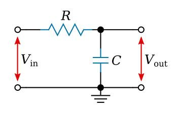
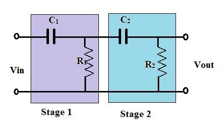
The simplest filter in existence is a single resistor wired with a single capacitor, with the audio signal applied across the pair and the output taken from across the capacitor. This two-component circuit is also known as a low-pass filter. Understanding why it works explains everything that follows.
A resistor resists the flow of electrical current at all frequencies equally. Now a capacitor behaves differently depending on frequency. At low frequencies, a capacitor barely lets anything pass at all. It charges up, holds its charge, and prevents the signal trying to flow through it. At high frequencies, because the signal reverses direction so rapidly, the capacitor never gets the chance to fully charge in either direction. It simply follows the rapid alternation of the signal, presenting very little resistance. The technical term for this kind of frequency-dependent resistance is impedance.
So if we wire a resistor and capacitor in series and take the output from across the capacitor, at low frequencies, the signal changes slowly. The capacitor has time to charge up fully in response to each half-cycle of the signal. Because it holds most of the circuit’s voltage, the output measured across it is large. The low-frequency signal appears at the output almost unchanged.
At high frequencies, the signal reverses direction so rapidly that the capacitor never finishes charging before it has to start discharging again in the opposite direction. It never accumulates significant voltage. Most of the signal drops across the resistor instead, and the voltage across the capacitor stays small. The high-frequency signal is reduced at the output.
Basically, the capacitor doesn’t let low frequencies pass through it but lets high frequencies pass through it. So, the high frequencies in the above figure go straight to the ground through the capacitor. This means high frequencies don’t appear at the output and low frequencies do and that’s a low pass filter.
High Pass Filter
High Pass Filter
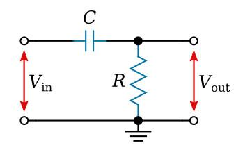
If we reverse the positions of the resistor and capacitor, and take the output from across the resistor instead, then at low frequencies, the capacitor’s impedance is high. This means it won’t let the low frequencies pass through. At high frequencies, the capacitor’s impedance falls, the resistor now carries most of the voltage, and the output is large. High frequencies pass. Low frequencies are attenuated. That is now a high-pass filter with just an exchange of capacitor and resistor positions.
This is the entire foundation of analog filter design. Every analog EQ ever built, from a Pultec EQP-1A to a Neve 1073 to an SSL 4000 series channel strip, is ultimately a network and combinations of these frequency-dependent impedance relationships, organized into circuits that modify the frequency response of the audio passing through them. Over time, the components change, the topologies grow more elaborate, inductors join the network alongside capacitors, active amplifier stages replace passive loss with active gain, but the underlying physics is always the same. Certain components present different opposition to different frequencies, and the ratio of those oppositions at the output determines what the filter does.
2.2 Cutoff Frequency and the Slope
Every filter has a cutoff frequency, also called the corner frequency. This is the frequency at which the filter’s attenuation begins to take effect. By convention, the cutoff is defined as the point where the signal is 3 dB below its level in the region the filter is passing. This means that say you have a 100 Hz signal at −3 dBFS and you put a high pass filter at 100 Hz, the signal will become −6 dBFS. It drops by 3 dB.
Below the cutoff of say a high-pass filter, the signal continues to be reduced as frequency decreases. We can plot how much each frequency reduces, to get a graph. The rate of that attenuation is the slope and is measured in decibels per octave. An octave is a doubling of frequency. A filter with a slope of 6 dB per octave reduces the signal by an additional 6 dB for every halving of frequency below the cutoff. A filter with a slope of 12 dB per octave reduces it twice as fast.
Second Order High Pass Filter
The slope of a filter is determined by its order. Each reactive component in the circuit, meaning each capacitor or inductor, contributes one order of filtering. A first-order filter has one reactive element and produces a slope of 6 dB per octave. A second-order filter has two reactive elements and produces 12 dB per octave. A third-order filter has three reactive elements and produces 18 dB per octave. Each additional order adds another 6 dB per octave to the slope.
Now, this relationship stays in both analog and digital filters. In analog circuits, the order is limited by the limitations of the component. This is because cascading many high-order filter stages introduces cumulative noise, distortion, and instability. Plus, the physical components become expensive and space-consuming. So for example, a 12th-order analog filter is quite difficult to build well. This means that most analog EQ high-pass and low-pass filters run between first order (6 dB per octave) and fourth order (24 dB per octave). Beyond that, the circuit compromises become audible.
2.3 Bell Curves and Shelves
A simple resistor-capacitor (R-C) pair only creates slopes. This means it is one frequency passband and one attenuated region, separated by a gradual transition. So in order to create the bell curves and shelves that define an equalizer, analog circuits end up using more elaborate arrangements of components, particularly something called inductors.
An inductor is simply a coil of wire. Its frequency behavior is the mirror image of a capacitor. While a capacitor resists slow changes in voltage, an inductor resists rapid changes in current. This means, at low frequencies, current changes slowly, the inductor offers little opposition, and it behaves almost like a plain wire. At high frequencies, current tries to change direction rapidly, the inductor fights that change, and its opposition becomes large. So the inductor’s impedance rises with frequency, while the capacitor’s impedance falls with frequency. This is why they are opposites.
If we wire an inductor and a capacitor together, something interesting happens at one specific frequency. At that frequency, the rising impedance of the inductor and the falling impedance of the capacitor reach a point where they interact in a way that either reinforces or cancels the signal very strongly. Below that frequency, the capacitor dominates. Above it, the inductor dominates. Right at it, the two forces act against each other in a way that produces a sharp peak or a deep notch in the circuit’s response. This is resonance, and the frequency at which it occurs is the resonant frequency of the inductor-capacitor (L-C) pair.
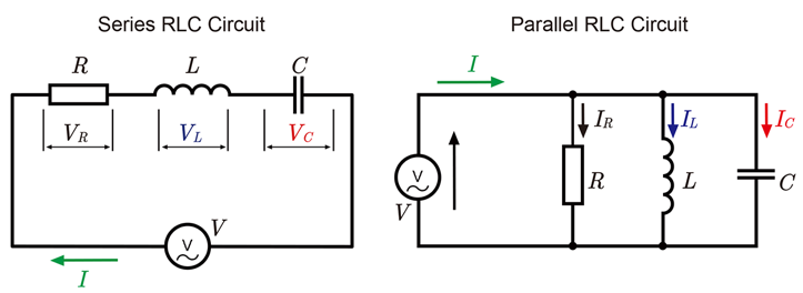
Series RLC Circuit (left) and Parallel RLC Circuit (right)
This is the origin of the bell filter in an equalizer. The resonant frequency of the inductor-capacitor combination becomes the center frequency of the bell curve. How narrow or wide the bell is, depends on how much resistance is present in the circuit to damp the resonance. A small amount of resistance produces a sharp, narrow bell with high Q. A large amount of resistance smears the resonance across a wider range of frequencies, producing a lower Q. Great. What is Q?
Q stands for Quality Factor, and interestingly, it comes from electrical engineering, not audio. When engineers were designing radio tuners, they needed a way to measure how well a resonant circuit could select one specific frequency and reject everything around it. A circuit that resonated sharply at exactly one frequency and ignored everything else was considered a high-quality tuner. And a circuit that resonated broadly and let in a wide range of frequencies around the target was considered a poor-quality tuner. This is why Higher Q is narrow and Lower Q is broader.
The gain at the center is determined by how strongly the resonance is driven relative to the rest of the circuit. In series, the impedance drops at the resonant frequency and current passes. In parallel, the impedance increases at the resonant frequency and the current drops.
Shelving filters use different configurations. These circuits are arranged so that the impedance relationships level out at a new value above or below the transition frequency rather than returning to the original level. The signal is either permanently lifted or reduced in a particular frequency region.
This is why early equalizers were made of inductors and capacitors rather than the active filter stages that followed. You see, the passive LC (inductor-capacitor) network could produce musically useful frequency response shapes using entirely passive components, with no power supply and no active gain. But the trade-off was signal loss at the insertion of the unit. Thus a passive equalizer always ended up reducing the output signal. The Pultec EQP-1A addressed this by adding a tube amplifier after the passive network to restore the lost level, which is why the Pultec has that particular character. The tube amplifier’s coloration is part of the sound.
2.4 Digital Filters
When digital audio systems arrived, engineers wanted to replicate what analog filters did in the digital domain. The fundamental challenge was that analog filters work because their components present different impedances to different frequencies in continuous, real-time electrical signals. Digital systems do not have continuous signals. They have streams of numbers, sampled at fixed intervals. There is no way a capacitor can respond differently to 100 Hz and 10,000 Hz in a digital system. This meant something different had to perform the equivalent function.
The answer, which Dan Lavry explained in his papers on filter operation, is that the equivalent of a frequency-selective impedance or the RLC circuit, can be achieved through mathematical processes applied to the stream of numbers. The digital filter does not have a capacitor that responds to frequency. Instead, it has a rule. That was to take the current sample, multiply it by a weighting value, take the previous sample and multiply it by another weighting value, add all those products together. The result of that addition is the output.
The weighting values are called coefficients. The number of past samples the filter examines is the filter length, and each sample position in that window is called a tap. The way those coefficients are shaped determines what the filter does to the frequency content of the signal. This is exactly as the values of the capacitors and inductors determine what an analog filter does.
A digital filter that is designed to replicate the behavior of a specific analog filter circuit uses coefficients that have been mathematically derived from the values of the analog components. By changing those coefficients we can change the filter, just as changing the capacitor or inductor values in an analog circuit changes the filter. Both produce the same result in the frequency domain.
2.5 Filter Coefficients
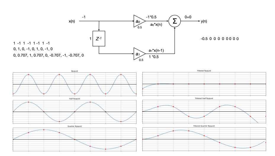
Filter coefficients: input waveforms (left) and filtered output (right)
According to me, Will Pirkle’s illustration of how digital filter coefficients work, in his book Designing Audio Effects in C++, is the best available one. Imagine the coefficients as a fixed row of numbered boxes laid out from left to right. The audio stream walks through those boxes one sample at a time. In the figure above, if we consider Nyquist frequency, those are 1, −1, 1, −1 and so on. The first sample 1 is multiplied by the coefficient here which is 0.5. That is then added to the previous one. Since there was none, the output would be 0.5. The next value is −1. That is multiplied by a0 which is 0.5 and the result is −0.5. The previous sample value was 1, and that multiplied by a1 which is 0.5 and that is 0.5. The sum is −0.5+0.5 = 0. The next sample is again 1 and it repeats.
That sum is repeated for each sample and is the output of the filter. In this particular example you can see that the filter completely attenuates the signal at Nyquist frequency. If we plot the signal values at each frequency, we get a slope. This is the slope of the filter and the point where the signal drops to −3 dB below the input value becomes the corner frequency.
The slope of a digital filter is determined by how many taps it uses. More taps mean a steeper, more accurate slope, for the same reason that more reactive components in an analog circuit produce steeper slopes. Each tap is the digital equivalent of one reactive element. A 16-tap digital filter achieves the equivalent of a 16th-order analog filter slope of 96 dB per octave, something completely impractical in analog hardware but straightforward in digital arithmetic. This is why the slope settings on a parametric EQ plugin are usually multiples of 6, and why the highest slopes available in digital EQ have no analog equivalent.
3 Filters and Phase
Phase is the part of audio that confuses us the most because it is invisible and largely inaudible in isolation, yet it somehow seems to affect everything. Every filter you use in an equalizer, introduces phase shift. Understanding what phase shift is and why it happens is very important in making decisions between minimum-phase, linear-phase, and natural-phase EQ modes.
3.1 What is Phase
We already know that sound is represented as a wave. At any given frequency, that wave goes up to a peak, comes back through zero, goes down to a trough, and returns to zero. This is one complete cycle and at 100 Hz it takes exactly 10 milliseconds, because the pattern repeats 100 times per second. Phase describes where in that cycle a particular frequency is at a particular moment in time.
If you have two identical sine waves at the same frequency and one is delayed relative to the other, they are out of phase. If the delay equals exactly half a cycle, the positive peak of one aligns with the negative trough of the other, and they cancel completely when summed. This is phase cancellation.
Now consider what a filter does. When audio passes through the coefficient computation described in the previous chapter, different frequencies arrive at the output with different amounts of delay. This is also why a one-sample delay introduces exactly 180 degrees of phase shift at the Nyquist frequency (the highest frequency the digital system can represent). The Nyquist has exactly two samples in it. So a 1 sample delay is exactly half a cycle. The delay that determines the filter’s cutoff behavior is the exact same delay that creates the phase shift.
3.2 Minimum Phase
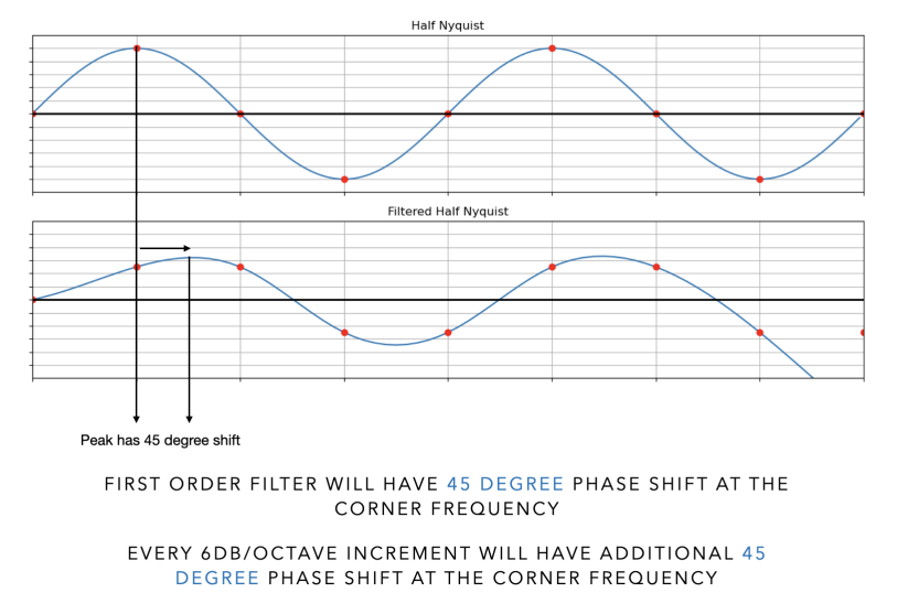
A first-order filter will have 45° phase shift at the corner frequency. Every 6 dB/octave increment will have additional 45° phase shift at the corner frequency.
Minimum phase simply means the filter introduces the least possible phase shift needed to produce its amplitude response. Every analog EQ ever made is minimum-phase. Every capacitor, every inductor, every resistor combination produces minimum-phase behavior. Analog components cannot look forward in time, or in other words have exact delay, so their response at any moment can only depend on what has already happened.
Whenever a filter changes the amplitude of a frequency, it also shifts the phase of that frequency by a specific amount. The two are linked. This means you cannot boost or cut a frequency in an analog circuit without also introducing a phase shift at that frequency. The amount of phase shift is the minimum amount that is mathematically possible to have, to produce that particular amplitude change. This is where the name comes from.
When you boost at 3 kHz on a Neve 1073, the frequencies around 3 kHz are slightly delayed relative to the frequencies further away from the center of the boost. At 3 kHz with a moderate Q setting, this delay is small. Research presented at the AES 124th Convention by Choisel and Martin found that phase distortion from filtering was difficult to detect in realistic listening situations in a room, even when present at levels that were audible in controlled headphone testing. The ear is not particularly sensitive to phase shift in isolation, particularly above 1 kHz.
The total phase shift from multiple minimum-phase filters in series can become more prominent. In a parametric EQ with six or eight bands all active, each band is adding its own phase shift at its own frequency. In mixing, where you might have a high-pass, two or three bell filters, and a shelf all active on a single track, the combined phase behavior is real, even if rarely audible in the context of the full mix.
Every analog filter ever made is minimum phase. There are no linear phase analog filters, because linear phase requires look-ahead. This means the filter must know what the signal is going to do in the future before it can produce its current output. Analog components cannot do this. A capacitor can only respond to what is happening to it right now.
This means that if you prefer the sound of analog gear, you are, in a way, preferring minimum phase behavior. Now, the phase shift that minimum phase filters introduce is not a flaw that maybe better analog design could eliminate. In fact, it is inseparable from what analog filters are. A plugin that models an analog EQ accurately will be minimum phase for the same reason the hardware is.
3.3 Linear Phase
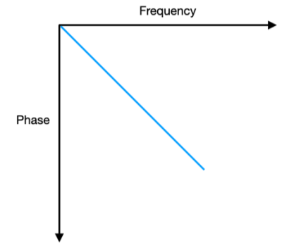
Linear-phase EQ is a capability that exists only in the digital domain. A linear-phase filter delays all frequencies by exactly the same amount. The frequency response is identical to its minimum-phase equivalent, but no frequency is delayed relative to any other. More specifically, we need a phase-shift response that changes linearly with frequency and this makes sense, because as the frequency increases a fixed phase shift corresponds to a gradually diminishing length of time since the wavelength is shorter, and thus we need more phase shift to compensate. This means if we plot all the values of phase against all the frequencies, it will be a straight line or linear slope.
This works because of a mathematical property of symmetric FIR (feed forward) filters. A feed-forward filter as the earlier example, will be linear-phase if its coefficients are symmetrical about their center. In a two-coefficient filter as in the earlier example, 0.5 and 0.5 is symmetrical. In a thousand-coefficient filter, the thousandth coefficient equals the first, the 999th equals the second, and so on. This symmetry guarantees that the phase response is perfectly linear across the entire frequency range, because the filter’s calculation is perfectly time-symmetric where it treats the future the same as the past.
The problem is that treating the future the same as the past requires actually knowing the future. How can you know tomorrow today? This is done by delaying a signal and waiting for the next. This is the source of the latency that linear-phase EQ introduces. The filter must buffer enough future samples to complete its symmetric computation before it can produce output. A filter with 1,000 coefficients must wait 500 samples before it has enough future context to begin outputting results. At 48 kHz, 500 samples is about 10 milliseconds. A filter with 10,000 coefficients introduces about 100 milliseconds of latency.
Linear-phase EQ also introduces something called pre-ringing. Now, because the filter’s computation extends symmetrically before and after the event, a sharp transient like a gunshot or a door slam will produce a faint ghost of its high-frequency content in the audio slightly before the main event arrives. This is the forward equivalent of the normal post-ringing that minimum-phase filters produce after a transient. For most material, this pre-ringing is inaudible. For completely isolated, sharp transients it can sometimes be detected on close listening.
3.4 Natural Phase
Natural Phase mode was something I saw in FabFilter’s EQ plugin. It uses a standard minimum-phase IIR (feedback) filter but applies a post-processing step that reshapes the phase response to minimize the whole frequency-dependent group delay variation that makes minimum-phase operation audible on complex, transient-rich material. So the result sits between minimum-phase and linear-phase. This means transients stay cleaner than with pure minimum-phase and without the latency or pre-ringing of linear-phase.
For most mixing tasks, Natural Phase is the most practically useful setting.
3.5 Which Phase to Choose?
Minimum-phase mode is the right choice for all single-track correction and shaping work like dialog, individual effects elements, music stems being processed individually. The minimum-phase behavior matches what every analog EQ does, and our ears are calibrated to it because it is what every analog studio tool in history has produced.
Linear-phase mode is a good choice when multiple parallel tracks must maintain their phase relationship through the EQ. When equalizing a multichannel bus where all channels must sum correctly to mono, or when applying a matched EQ across all channels of a 7.1.4 stem, minimum-phase processing applied identically to channels with different content produces different phase responses in each channel. When those channels are summed, the result is comb filtering and imaging artifacts. Linear-phase processing applied identically to all channels produces identical delay across all of them, preserving inter-channel relationships. But bear in mind that it does create more latency and delay.
Natural Phase is the right choice when you want the tonal contribution of a minimum-phase filter but are working on material where the cumulative group delay of a complex EQ setting is audible as slight softness in the transient texture.
When you run parallel processing, meaning you split a signal, process one copy, and sum it back with the original signal, you introduce a phase problem that is easy to miss and this is important to understand.
You see, every minimum phase filter changes the phase of the signal as well as its amplitude. When the processed (wet) signal is summed with the original (dry) signal, the frequencies where phase has shifted because of the processing, now exist in the wet at a different phase than the original dry one. Depending on the degree of phase shift at each frequency, they can partially cancel or partially reinforce. The result is comb filtering which is a series of peaks and dips. This can color the summed signal in a way that neither the wet nor the dry signal produces on its own.
The correct solution is to run the dry signal through an all-pass filter on the dry that matches the phase trajectory of the wet signal before the two are summed. This way the wet and dry signals arrive at the summing point with the same phase relationship, and the comb filtering disappears. This is because the dry has been phase-shifted to match the wet signal.
3.6 Gibbs Phenomenon
When a filter removes a band of frequencies from a signal, it is cutting the frequency spectrum at a sharp boundary. Now, a perfectly sharp boundary in the frequency domain, meaning a filter that passes everything below a certain frequency and blocks everything above it completely, is mathematically impossible to achieve in finite time. The attempt to approximate it produces small oscillations called ripples on either side of the boundary. These ripples are called the Gibbs phenomenon. They appear wherever there is a sharp discontinuity in a signal or a sharp edge in a filter’s frequency response.
In a minimum phase filter, these ripples appear only after the edge, meaning after a transient or after the cutoff point. You will see a small oscillation that decays over time following the sharp event. In a linear phase filter, the computation is symmetric around the point of processing, treating past and future equally. This symmetry distributes the ripples on both sides of the edge. So, some appear before the transient and some after. The ripples that appear before the main event are what engineers call pre-ringing.
The steeper the filter, the worse the Gibbs phenomenon becomes. A gentle filter slope approximates the frequency domain boundary gradually and produces small, brief ripples. A very steep filter, close to a brickwall response, requires a very long computation window to approximate the sharp boundary accurately. That long computation window pushes the pre-ringing further back in time before the transient. On a gentle filter with a short impulse response, the pre-ringing is a few samples long and completely inaudible. On an extreme brickwall linear phase filter with a very long impulse response, the pre-ringing can extend several hundred milliseconds before the transient and may become audible on sharp, isolated sounds at low frequencies.
This is why brickwall linear phase filters are genuinely problematic in a way that gentler linear phase filters are not. The problem is not linear phase itself. It is the combination of linear phase with an extreme slope, because the extreme slope demands a long enough impulse response to push the Gibbs ripples far enough back in time to be heard. For the moderate slopes used in most EQ work, pre-ringing from the Gibbs phenomenon remains well below the threshold of audibility.
The thing is you cannot fix this from outside the plugin by say inserting an all-pass filter on the dry signal. You would need to know the exact mathematical implementation of the developer’s filter to apply matching phase compensation yourself, which is impossible. When a developer has built phase compensation into the plugin’s wet-dry mix, use their mix knob rather than creating your own parallel path in the DAW. This is also why some plugins sound better used as sends than as inserts. When used as a send, the wet signal returns alongside the original dry track in the DAW. If the plugin has not phase-compensated its dry path, the parallel combination at the DAW summing bus will comb-filter.
4 FIR and IIR Filters
There are two fundamental architectures that exist for digital filters. Every digital EQ uses one or the other, or a combination of both. These are FIR (Finite Impulse Response) and IIR (Infinite Impulse Response) filters. The difference between them teaches us everything about latency, phase behavior, computational cost, and sonic character.
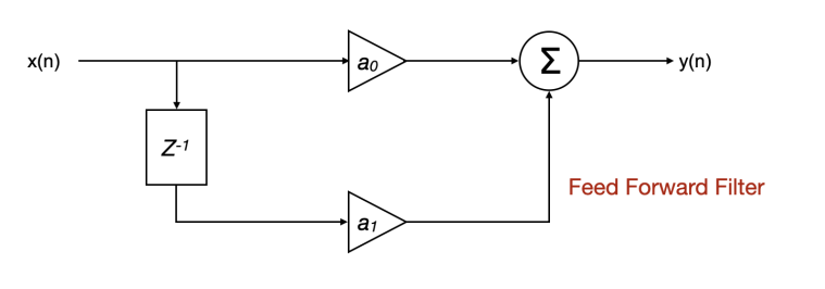
4.1 FIR (FeedForward Filter)
1st Order FIR
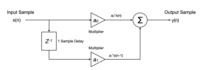
A FIR filter is essentially a feed-forward filter. This means that signal flows from the input to the output in one direction only. There is no feedback path. Nothing from the output ever goes back to the input. The filter looks at the current input sample and a specific number of past input samples, multiplies each by a coefficient, and sums the results. The output is calculated, delivered, and that is the end of the process for that sample. The filter then moves on to the next one. In the above diagram, a0 and a1 are filter coefficients, Z⁻¹ is the 1 sample delay. Each sample delay is a tap. So the above is a 1st order FIR because it has one tap.
Now, why is it called Finite Impulse Response? It simply means the response of an impulse is finite. Since nothing ever feeds back, the filter’s response to any single input event is finite. Feed it an impulse (a single sample at value 1, all others at value 0), and the output will show a brief flurry of non-zero values as the impulse travels through the coefficient window, and then return to exactly zero once the impulse has passed through all the taps. After that, silence. The response is finite in time. Thus the name Finite Impulse Response.
When you send a sine wave through a multi-tap FIR filter, each tap receives the same sine wave but shifted by one sample period. Adding those delayed copies together either reinforces or cancels the sine wave at each frequency, depending on the phase relationship between the delayed copies. The set of coefficients determines the outcome at every frequency simultaneously. The coefficient profile is the frequency response, directly.
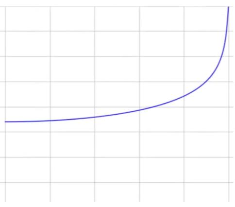
Amplitude vs Frequency for 1st order FIR
The computational cost or CPU load of a FIR filter will scale directly with the number of taps. A 1,000-tap FIR filter requires 1,000 multiplications and additions per sample. At 48 kHz stereo, that is nearly 100 million multiplications per second. A linear-phase EQ with steep slopes and low cutoff frequencies might require tens of thousands of taps, demanding hundreds of millions of operations per second per channel. This is why linear-phase EQ plugins have historically required significant CPU.
4.2 Slope of a Filter
The number of taps (number of coefficients in parallel) in a FIR filter directly determines how steep and how accurate its transition between passband and stopband can be. Passband is the frequency range that is let through and stopband is the frequency range that is cut off. A filter with very few taps can only produce gentle slopes. Each additional tap gives the filter more information about the history of the signal and allows it to make finer frequency distinctions.
A 9-tap FIR filter used as a 15 kHz low-pass at 44.1 kHz produces a frequency response that is flat to roughly 4 kHz, then gradually rolls off, reaching only about 14 dB of attenuation at 20 kHz. A 500-tap version of the same filter is flat to 15 kHz, then drops 100 dB at 16 kHz and 140 dB at 22 kHz. The computational cost rose from 9 multiplications per sample to 500, but the filter’s performance improved by an order of magnitude in terms of stopband attenuation.
This is why some linear-phase EQ plugins offer a quality or resolution setting. Higher quality settings use more taps. This does mean more latency but it offers more accurate frequency responses.
4.3 IIR (Feedback Filter)
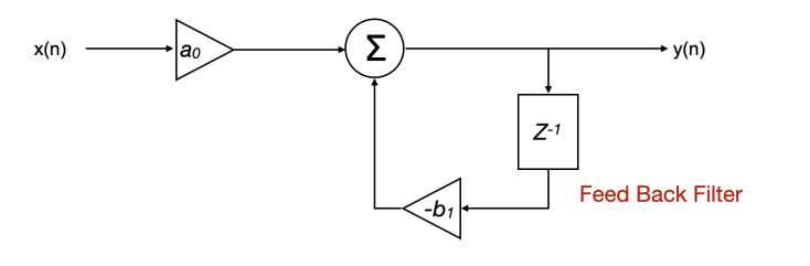
1st Order IIR
An IIR filter is a feedback filter. As before, the signal flows forward from input to output, but the output is also fed back into the calculation as additional input for the next sample. The filter computes each output sample not only from the current but also from past outputs.
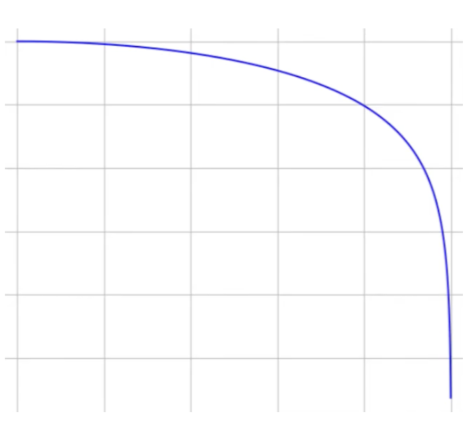
Amplitude vs Frequency for 1st order IIR
This feedback loop is why the IIR filter’s response to an impulse can theoretically last forever. This is where the name Infinite Impulse Response comes from. The response to an impulse can be long. If we send a single impulse, the feedback path keeps recycling a diminishing fraction of the output back into the input at every subsequent sample time. The signal decays exponentially toward zero but never actually reaches it. In practice, the ringing decays to a level below the noise floor within a few milliseconds for a well-designed audio filter, but the mathematical possibility of infinite duration is where the name comes from.
The interesting part is that this feedback behavior allows IIR filters to do something FIR filters cannot do with lesser CPU load. And that is to create resonant peaks and very rapid transitions between passband and stopband without a huge number of taps. Even just a second-order IIR filter (two forward taps and two feedback taps, five multiplications and four additions per sample) can produce a bell filter with steep Q, a resonant peak, and a specific phase trajectory. An FIR filter producing the same frequency response would require hundreds of taps.
IIR filters are the digital equivalents of analog circuits. The mathematical descriptions of resistor-capacitor networks, inductor-capacitor networks, and op-amp feedback configurations all can be converted directly into IIR filter designs. When a plugin manufacturer says their equalizer is modeled on specific analog hardware, what this means under the hood is that they have taken the circuit equations for that hardware, applied a standard mathematical transformation called the bilinear transform, and implemented the result usually as an IIR filter. The resulting filter behaves in the same way as the original circuit, including its phase response.
IIR filters are inherently minimum-phase. The feedback that makes them computationally efficient also locks them into minimum-phase behavior. Because of the way it fundamentally works, there is no way to make a standard IIR filter linear-phase without post-processing.
4.4 Poles and Zeros
There are two interesting concepts you might hear when reading on filters. They are Poles and Zeros.
A zero is a frequency where the filter’s output drops to nothing. This is like what we saw in the FIR Amplitude vs Frequency graph earlier. The signal is cancelled completely at that point. Sometimes on a frequency response plot it appears as a notch cutting all the way to silence. The name is literal. Zero is the mathematical expression describing the filter goes to zero at that frequency.
A pole is the opposite. It is a frequency where the filter’s response wants to go to infinity. An example is what we saw in the IIR graph earlier. In a real, stable filter it never gets there. In design, the pole of a filter is placed just short of that point by mathematically calculating the coefficients, but the tendency toward infinity is what creates a peak in the response. The closer the pole sits to that limit, the sharper and taller the peak. If we move it further away, the peak broadens and flattens. The Q of a bell EQ band is directly controlled by this distance. This means tight poles produce high Q narrow peaks, loose poles produce low Q broad curves.
Every filter is a combination of poles and zeros working together. A low-pass filter uses poles near the cutoff frequency to shape the rolloff and zeros in the stopband to kill the high frequencies. A bell EQ boost uses a pole pair to create the peak and a zero pair to pull the response back to flat on either side. A notch filter places a zero precisely at the problem frequency and a pole just beside it to keep the surrounding response intact.
This is useful in practice because the pole and zero locations completely determine the filter’s behavior. And it does this not just for the amplitude response but the phase response as well. Moving a pole changes both simultaneously, which is why you cannot adjust the shape of a minimum phase filter without also changing its phase.
If we extend this to minimum phase and linear phase, most professional EQ plugins today use both architectures. The minimum-phase mode uses IIR filters and these are computationally inexpensive, zero latency, minimum-phase behavior that matches what every analog hardware unit produces. The linear-phase mode switches to FIR filters which has more CPU demand, latency-inducing, but perfectly linear phase. As mentioned, FabFilter’s Natural Phase mode uses IIR filters with a phase-correction post-process. Some plugins apply the filter twice in opposite directions through the audio offline, which produces linear-phase behavior from IIR filters at the cost of real-time processing.
5 Families of Filters
When you set a high-pass filter to 100 Hz at 12 dB per octave, you have made two decisions. One is where the filter acts, and the other is how steeply it acts. But we usually don’t decide how this is done. That decision is made by the filter family. You see, the filter family determines the shape of the transition between what passes and what is blocked, and it determines how the filter behaves. Two filters can have the same cutoff frequency and the same order and still sound different, because they belong to different families.
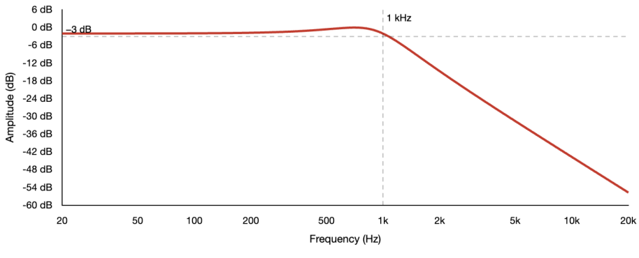
The Butterworth filter, developed by British engineer Stephen Butterworth in 1930, has one absolute priority. Every frequency in the passband must be treated equally. No frequency should be louder or quieter than any other. This means the passband must be completely flat. This property is called maximally flat, and no other filter design of the same order can produce a flatter passband.
But the cost of that decision is that the transition band is the widest of the amplitude-focused filter families. As you see in the image, the filter does not make sharp changes near the cutoff. It eases gradually into its attenuation. At the cutoff frequency it has attenuated the signal by exactly 3 dB, and the curve rolls off smoothly from there.
If we send white noise through a Butterworth low-pass at 100 Hz, everything above 100 Hz comes through at equal level. Right at 100 Hz it is 3 dB down. Below 100 Hz it rolls off smoothly. On a spectrum analyzer the passband is a perfectly flat line and the transition is a smooth curve. Now if we send a sharp transient through the same filter, the Butterworth settles cleanly with a single small overshoot and returns to stability quickly. The attack of the transient is preserved, with only a small rounding at the leading edge. This moderate transient behavior, although neither the best nor the worst of the families, is part of why the Butterworth is the default in almost every mixing EQ. It sounds like nothing is happening except the unwanted low frequencies disappearing.
The Chebyshev filter is named after a mathematician and not the inventors. It is interesting because the Russian mathematician Pafnuty Chebyshev was working on the mathematics of designing a linkage that converts rotary motion to linear motion with minimum deviation. The polynomials called Chebyshev Polynomials, also happened to be a solution to how do you get the steepest possible rolloff for a given filter order while keeping the passband behavior controlled.
Now, actually Chebyshev filters make a different priority choice. It is more like: I want to block frequencies near the cutoff more aggressively than the Butterworth can. I want the transition band to be narrower, so that frequencies just below the cutoff are attenuated more decisively.
Now, to achieve that with the same filter order, something has to be compromised. This is where the Chebyshev passband is not flat. It ripples, oscillating a fraction of a dB above and below the target level in a regular wave pattern across the frequencies being passed. The frequencies in the passband are not all treated equally. Some come through fractionally louder, some fractionally quieter.
Here, if we send white noise through a Chebyshev low-pass at 100 Hz, the spectrum analyzer shows that below 100 Hz the line is no longer flat. It oscillates slightly, perhaps 0.5 dB up and down, in a regular repeating pattern. The transition above 100 Hz is actually steeper than the Butterworth, reaching deeper attenuation at frequencies closer to the cutoff. But the passband has that characteristic ripple pattern running through it.
Now if we send that same sharp transient through, the Chebyshev behaves quite different compared to the Butterworth. The ringing in its frequency response translates directly into ringing in its time response. The transient produces a sustained oscillation after its attack, a series of decaying echoes that take several milliseconds to settle. In a real audio context, a gunshot or a sharp consonant processed through a steep Chebyshev high-pass can produce a subtle artificial ring after the main event. This is why Chebyshev filters are not used in general-purpose mixing EQs, and why the Butterworth’s gentler transition actually serves audio better despite being technically less efficient.
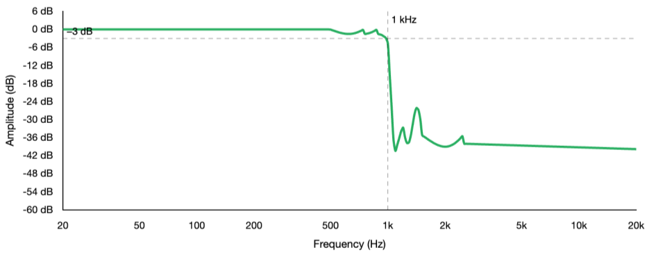
The elliptic filter takes the Chebyshev idea to its logical extreme. It allows ripple in both the passband and the stopband simultaneously, and in exchange it achieves the steepest possible transition from passband to stopband of any filter at a given order. No other filter design can match the elliptic for transition steepness when the filter order is fixed.
The elliptic filter can reach complete, total rejection at specific individual frequencies in the stopband. We can even see this on a spectrum analyzer as deep, narrow notches at specific frequencies beyond the cutoff. This is also why elliptic filters are used in analog-to-digital converters. If you think about it, the anti-aliasing filter must provide near-complete rejection at the Nyquist frequency to prevent frequencies above it from folding back into the audio as spurious tones. The Brickwall setting in FabFilter Pro-Q 4 uses this approach, and it is the correct choice whenever you need a hard spectral limit, such as keeping content strictly below 120 Hz for the LFE channel.
Now, there is an interesting way to understand the relationship between all these families. The elliptic filter is actually the most general case. If you design an elliptic filter and remove the stopband ripple, you get a Chebyshev Type I. If you remove the passband ripple instead, you get a Chebyshev Type II. If you remove ripple from both bands, you get a Butterworth. The families are all linked with elliptic at one extreme and the Butterworth at the other.
5.4 Bessel
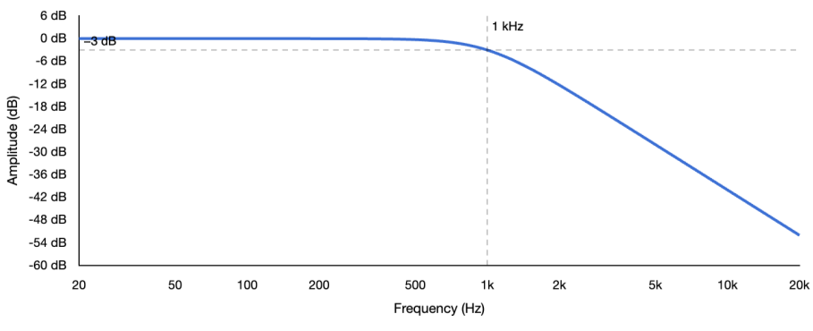
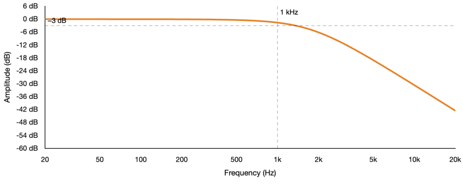
Bessel Filter – 2nd order, low-pass, 1 kHz cutoff
This filter gets its name from a German Astronomer Friedrich Bessel, who in the early 19th century, was computing the gravitational influence of planets on each other’s orbits. In his work, the differential equation that kept appearing in those calculations produced a family of solutions now called Bessel functions. W.E. Thomson in 1949 made the connection that these functions can create a maximally flat group delay where all frequencies are delayed by the same amount through the filter. This means the phase response is linear and the waveshape of a complex signal is preserved as cleanly as possible, and the Bessel Filter was formed.
So, the Bessel filter actually makes the opposite priority choice from the Chebyshev. It gives up transition steepness to make sure that every frequency passing through the filter is delayed by exactly the same amount. You could say this is, in a way, the analog world’s closest match to a linear phase filter but it achieves this only in the passband where relationships between frequencies are perfectly preserved.
Every other filter family delays different frequencies by different amounts. A low-frequency component and a high-frequency component entering the filter at the same moment emerge at slightly different moments. The Bessel filter eliminates this within the passband.
The result of this in the time domain is dramatic. So if we send a sharp transient as before through a Bessel filter, it settles almost immediately with no overshoot and no ringing. While the Chebyshev rings for several milliseconds and the Butterworth shows a single small overshoot, the Bessel actually reproduces the transient’s shape almost perfectly.
This is why the Bessel is unique. It cleanly preserves timing of the signal that passes. When we send white noise through a Bessel high-pass at 100 Hz and compare it on a spectrum analyzer to a Butterworth at the same setting, the Bessel will show more low-frequency content coming through near the cutoff. The transition is noticeably softer and more gradual. It is actually a less decisive filter in terms of amplitude. But the attack of every transient that passes through it arrives intact.
In audio EQ you rarely see pure Bessel designs. This is because a Bessel filter needs a much higher order to do what a Chebyshev does. But where they show up more often is in anti-aliasing filters, crossover networks where transient coherence matters, and instrumentation where waveshape preservation is the primary requirement.
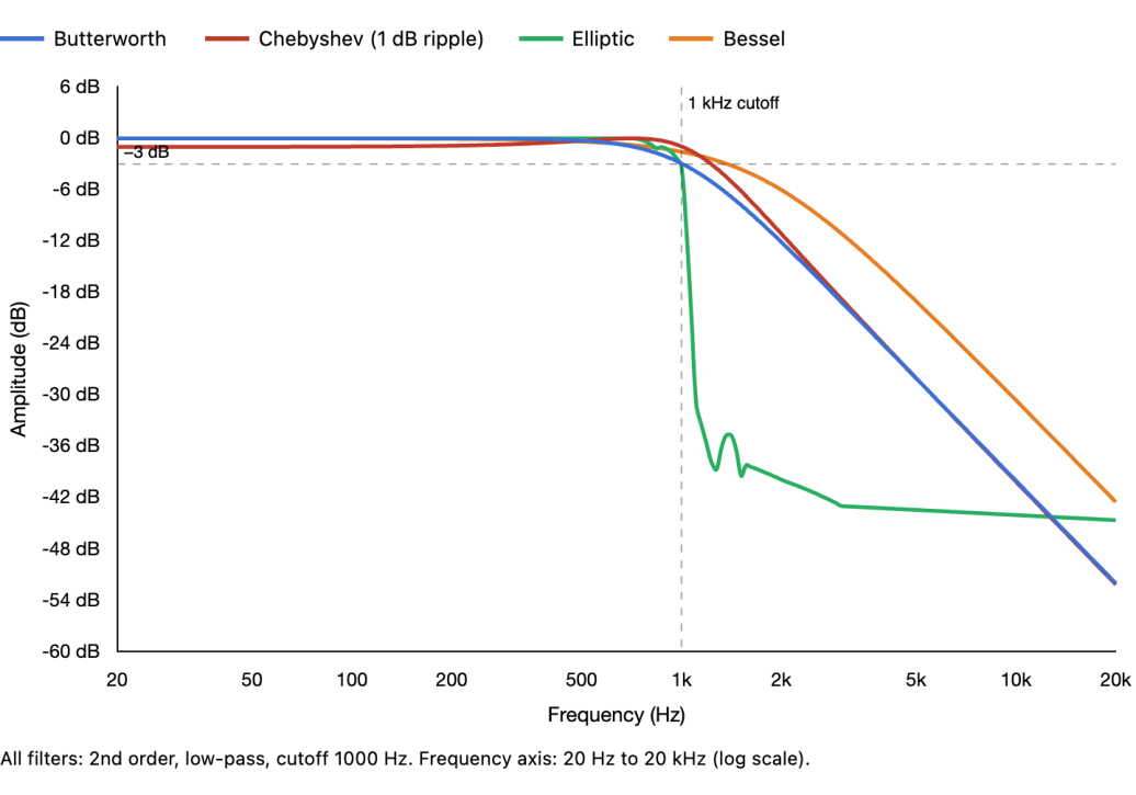
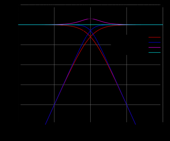
All filters: 2nd order, low-pass, cutoff 1000 Hz. Frequency axis: 20 Hz to 20 kHz (log scale).
In a way, the term frequency response is a misleading name for what a filter does, because every filter changes two things simultaneously. Amplitude and Phase. These two are inseparable in any filter. When you boost at 3 kHz on a parametric EQ, the frequencies around 3 kHz are not just louder in the output, but they are also slightly delayed relative to the frequencies further from the boost. The amplitude change and the phase change happen together, always, in every filter you have ever used.
6 Types of Filters
Now, that we have seen the family of filters, let’s look at some of the common types of filters built from them that exist today.
6.1 High-pass Filter
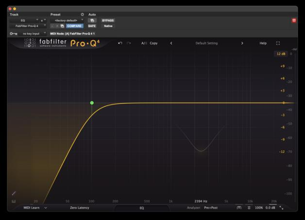
A high-pass filter passes frequencies above its cutoff and attenuates everything below. So, as an example, a high-pass filter on a dialog track is almost always the first EQ decision. Anything below 80 Hz in a voice recording is almost certainly handling noise, air conditioning rumble, electrical hum, or proximity effect buildup from a close lav mic. A high-pass at 80 to 100 Hz removes this without touching the voice itself.
The resonance setting at the cutoff frequency affects the character of the transition. A filter with no resonance (Butterworth-like) transitions smoothly from the passband to the attenuated region with no bump at the cutoff. A filter with resonance adds a small peak just above the cutoff before rolling off, adding a subtle bite or presence to the transition. This is part of why different high-pass filters sound different even at the same cutoff frequency and slope setting.
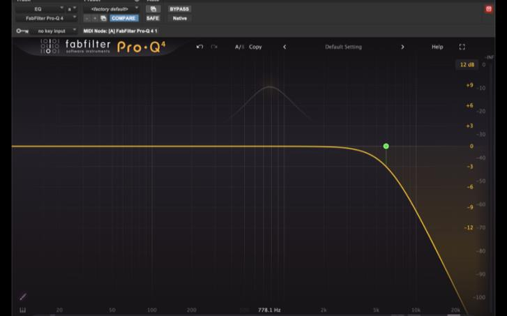
6.2 Low-pass Filter
A low-pass filter passes frequencies below its cutoff and attenuates everything above. As an example, rolling the high end off a gunshot makes it sound further away because air absorbs high-frequency content significantly over distance. Now, of course the amount of absorption depends heavily on temperature and humidity. Say at 10 kHz under typical outdoor conditions it can range from around 4 to 10 dB per 100 metres, with dry air absorbing far more than humid air. This is why a gunshot or explosion heard across a large open space, sounds dull and low-heavy compared to the same sound at close range. Low-pass filters on ambience tracks push them back in a scene. On music stems in complex action sequences, a low-pass can remove the high-frequency congestion that occurs when music, effects, and dialog all compete for the same spectral real estate.
6.3 Bandpass Filter
A bandpass filter passes a specific band of frequencies and attenuates everything above and below. It is a high-pass and a low-pass filter in series. The classic telephone bandwidth runs from roughly 300 Hz to around 3,000 Hz, so a bandpass filter with those cutoff points applied to a voice creates a credible telephone sound. The steepness of the edges controls how telephone-like or how harsh the effect sounds.
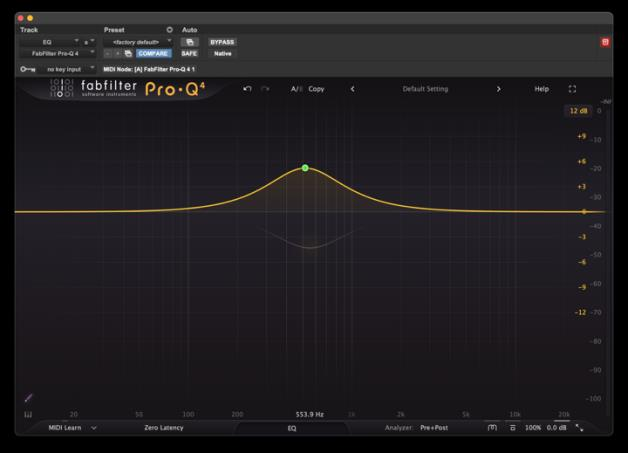
6.4 Bell Filter
The bell filter is named for its shape on a frequency response plot. It is a symmetrical curve that rises to a peak (on a boost) or falls to a notch (on a cut) at the center frequency, then falls away symmetrically on either side. The controls are center frequency, gain (positive or negative), and Q (bandwidth). Q stands for Quality factor, and it describes the ratio of the center frequency to the bandwidth at which the filter is 3 dB away from its maximum effect. Narrow-Q bell filters chase down the specific resonant frequencies that make a particular voice sound honky, nasal, or boxy. A broader bell cut at 300 to 500 Hz might reduce the overall muddiness of a lav recording without targeting a specific resonance. Narrower addresses the problem more precisely but sounds more processed if overdone. Broader sounds more natural but affects more of the surrounding spectrum. It is good to note that Q can’t always be defined exactly with bell curves because sometimes the boost or cut is less than 3 dB.
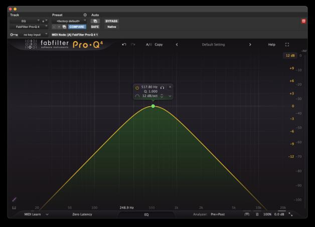
6.5 The Shelf Filter
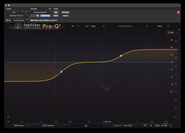
A shelf filter affects all frequencies above (high shelf) or below (low shelf) a chosen frequency, boosting or cutting that entire region to a flat new level. Unlike a bell filter, a shelf’s effect does not fall away with distance from the center frequency. Instead it levels off at the boost or cut amount and stays there. Shelves are like the bread and butter of tonal shaping. They are the ones adding air to dialog with a high shelf boost, warming a thin ADR track with a low shelf boost, or reducing the weight of distant room tone with a low shelf cut. The Q parameter controls the shape of the transition region. A low Q produces a broad, gentle transition. A high Q produces a steeper, more immediate step. Some shelf designs allow a variable tilt so the shelf can continue rising or falling beyond the set frequency rather than leveling off flat, producing more dramatic tonal shapes.
6.6 The All-pass Filter
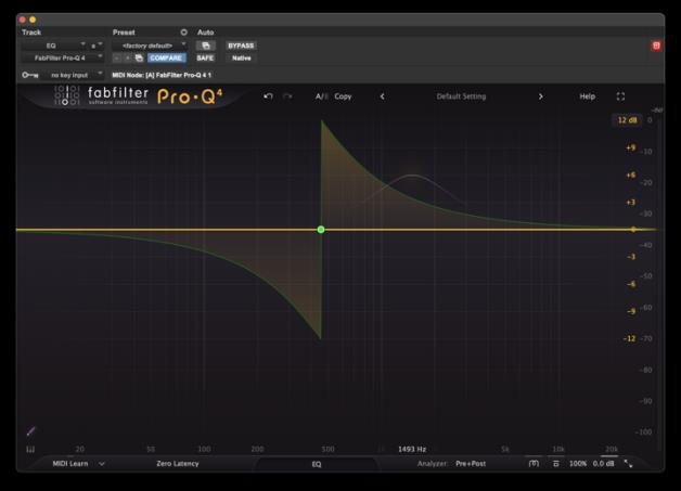
The all-pass filter passes all frequencies at equal amplitude. Its frequency response plot is a perfectly flat line. What it changes is the phase relationship between frequencies. It introduces a phase shift that varies with frequency, delaying some frequencies relative to others without changing their level at all. All-pass filters are used inside equalizers to shape the phase response independently of the amplitude response. They are the mechanism behind the Natural Phase and Analog Phase modes in digital EQ plugins. FabFilter Pro-Q 4 includes an explicit all-pass band type, allowing engineers to add phase correction without any amplitude change. A trick of adding an all-pass filter matched to the phase part of a specific analog circuit model can sometimes make a digital EQ sound slightly more like its hardware counterpart, even at flat gain settings.
6.7 The Notch Filter
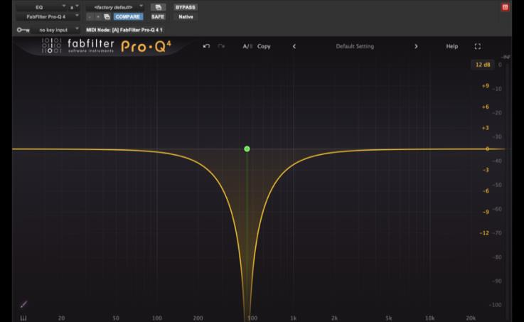
A notch filter is a bell filter with a very high Q (often above 10) applied as a cut. The result is an extremely narrow, deep cut at a single frequency, leaving everything on either side effectively untouched. So a 50 Hz notch removes mains hum from a European recording, a 60 Hz notch from an American recording. An 18 kHz notch removes the high-pitched whistle from old fluorescent light fixtures on location recordings. A precisely tuned notch at the resonant frequency of an actor’s wristwatch or jewelry can reduce the offending tone without touching the surrounding dialogue.
6.8 Proportional Q
A standard bell filter applies the same Q regardless of how much you boost or cut. Proportional Q (introduced by Saul Walker in the API 550A in 1967) changes the Q automatically in response to the gain amount. At small amounts of gain, the Q is low and the filter is broad. As you increase the gain, the Q rises and the filter becomes narrower. This prevents extreme settings from sounding unnaturally resonant. At 2 dB of boost, you are shaping a broad, musical region. At 12 dB of boost, the filter has tightened itself to keep the result from sounding like a resonant spike. This is part of why the API 550A has a reputation for sounding punchy and fast without becoming harsh at extreme settings.
6.9 Linkwitz-Riley
Linkwitz-Riley crossover design
The Linkwitz-Riley is not really a filter but a specific crossover design built from Butterworth filters. On the low-pass path, two Butterworth low-pass filters of the same order are cascaded in series. On the high-pass path, two Butterworth high-pass filters of the same order are cascaded in series. Both paths share the same corner frequency. There is a reason this is done.
At the crossover frequency, each individual Butterworth filter is 3 dB down by definition, because the corner frequency is the point where a filter attenuates the signal by 3 dB. Cascading two Butterworth filters doubles the attenuation in dB at every frequency, so each path is 6 dB down at the crossover. Six dB of attenuation means the amplitude is exactly half or 0.5. Because the Linkwitz-Riley construction also ensures that the high-pass and low-pass outputs are in phase with each other at the crossover point, when the two paths are summed, 0.5 plus 0.5 equals 1.0. Unity gain. This is how the crossover works with no gain loss in this design.
This perfect summation is why Linkwitz-Riley crossovers are the standard design in multiband compressors, multiband EQs, and speaker management systems. Any time a signal is split into bands and recombined, the crossover must sum to unity or the recombined signal has a frequency response error at every crossover point.
This actually is very important whenever a signal is split into bands and then recombined. In a multiband compressor for example, the signal is split into bands, each band is compressed separately, and the bands are summed back together. If the crossover filters do not sum perfectly, the recombined signal has a bump or a hole in the frequency response at every crossover point. Linkwitz-Riley crossovers guarantee that does not happen. The most common version is the fourth-order Linkwitz-Riley, which is two second-order Butterworth filters cascaded in series, producing 24 dB per octave with perfect summation at the crossover frequency. The Avid Pro Multiband compressor uses an eighth-order Linkwitz-Riley, which is two cascaded fourth-order Butterworths on each path, producing a 48 dB per octave slope. The steeper slope gives tighter band separation between the compression zones, which is why multiband compressors intended for mastering use higher-order crossovers.
7 The Color of Analog EQ
The most common mistake we make when thinking about EQ, is believing that a flat-positioned equalizer is sonically transparent. In analog circuits, this is not really true. Audio passing through an EQ’s circuitry is influenced by every component it encounters. This includes the input and output transformers, the operational amplifiers or discrete transistor stages, the passive components in the filter networks, and the coupling capacitors in the signal path. In fact, it is a large part of why specific EQ designs became famous.
7.1 Transformers
Transformers are wire coils wound around a magnetic core, used at the input and output of many vintage and boutique EQs to provide electrical isolation and impedance matching. Transformers saturate. This means they produce harmonic distortion when the signal level or low-frequency content drives them beyond their linear range. The distortion produced is predominantly second and third harmonic. Second harmonic gives a smooth, even character. Third harmonic adds a slightly more complex, firm quality. One thing to keep in mind is that these harmonics create what is called Intermodulation Distortion as well sometimes. These are not necessarily musical in context and sometimes in comparison to the quality of even vs odd harmonics, these could be more damaging in comparison.
The classic Neve 1073 channel strip uses Marinair transformers at its input and output, and the interaction between the signal and those transformers is a primary source of the 1073’s famous sonic character. When audio passes through a 1073 with flat EQ settings, it will return with more weight in the low end, more presence in the upper midrange, and a silky quality in the highs. The EQ circuitry adds further color when engaged.
7.2 Inductors
Inductors are coils of wire around a magnetic core that present frequency-dependent resistance. At low frequencies, an inductor passes signal freely. At high frequencies, it resists the signal. This makes inductors naturally suited for building filter circuits, and they were the primary means of building broad, gentle shelf and bell curves before operational amplifiers became cheap and reliable. Inductors saturate nonlinearly when the signal pushes them hard, contributing harmonic content to the sound. The positive half of a signal and the negative half of the signal push the saturation of the core equally in opposite directions. When it is saturated, it means the signal gets compressed. This compression is equal in both directions. This means it is symmetrical. And symmetrical compression produces odd-order harmonics – primarily the 3rd and 5th. Even-order harmonics, the kind you get from asymmetrical saturation in single-ended tube stages, are generally considered more musical. But inductor saturation in audio circuits is gentle. The 3rd harmonic dominates without the higher odd-order content that makes distortion sound harsh. That gentle saturation, combined with the natural high-frequency rolloff of the inductor and its soft, program-dependent compression behavior, is what gives inductor-based gear its warmth. It’s because the overall character of the nonlinearity sits in a sweet spot.
As Rupert Neve Designs describe their custom-wound inductors, when they saturate, they produce beautifully musical harmonics that add smooth, polished tone. This is precisely why a Neve EQ sounds fundamentally different from an op-amp-based EQ with an identical frequency response curve. The filter network is itself a tone-shaping circuit, not merely a mathematically neutral frequency modifier.
7.3 Class-A Circuitry
To understand this, we need to know what a transistor is and how it works.
Think of a garden hose where you pinch the end of the hose in it. The water pressure comes from the tap so let’s call that the power supply. The pinch controls how much water gets through. Your fingers control the pinch. A small physical effort from you determines a large flow of water. Now, the energy comes from the tap, not from you. You’re just operating the gate.
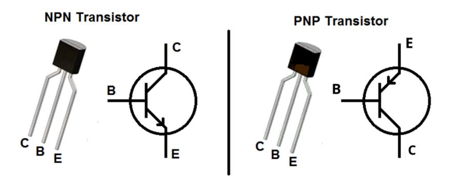
NPN Transistor (left) and PNP Transistor (right)
A transistor works the same way. It has three terminals. A large current path from collector to emitter (the tap), and a control terminal called the base (the pinch). A small current into the base opens or tightens the gate for the large current. The ratio between the two is the transistor’s gain. This is typically 100 to 500, meaning a 1 milliamp nudge at the base changes 100 to 500 milliamps at the collector. Now, our audio signal goes into the base. The transistor translates those tiny variations into proportionally larger variations at the collector. Same shape, bigger movement. So you see, the transistor isn’t generating energy. What it does is it’s using your small audio signal as an instruction for shaping a larger flow of energy that the power supply is already providing.
But what does the transistor do when there is no signal?
In a Class-B design, the transistor idles. It conducts only when the signal pushes it. A signal is made of positive and negative cycles. So if we use two transistors with one for positive swings, one for negative, we cover the full waveform while keeping each transistor off for half the cycle. This is great. But at the moment the signal crosses zero, we have a problem. Each transistor needs about 0.6 volts across its base-emitter junction before it starts conducting. So there is a dead zone which is roughly 1.2 volts wide, where the signal is too small to turn on either transistor. The output just goes silent in that window. This is crossover distortion. It chops into the waveform twice per cycle, right at the zero crossing. This produces high-order odd harmonics and sounds harsh in a way that is difficult to ignore especially at low levels.
Class-A eliminates this by refusing to let the transistor idle. A DC bias is sent that holds the transistor in the middle of its conducting range at all times. The signal arrives and moves that operating point up and down, but the transistor never approaches the off condition. Zero crossing isn’t an issue at this point because the transistor doesn’t switch – it just modulates.
But the cost of this is heat. That DC bias current flows continuously regardless of signal level, and most of it ends up becoming thermal energy rather than audio output. So what you end up getting in return is a transistor operating continuously in its most linear region. Now, a transistor has a transfer curve that is slightly curved rather than perfectly straight. That curvature colors the signal in a specific way. The distortion it generates are mostly the octave above the fundamental and is second harmonic. This second harmonic distortion is what your ear associates with warmth and fullness. It’s what a tube produces and what an inductor produces when it saturates.
At low drive levels, the Neve 1073’s Class-A stages produce this beautiful second-harmonic character. If we push the input harder, the operating point moves further around the curve, engaging higher-order terms and producing a richer, more complex harmonic mix. This is still musical, because even harmonics remain dominant, but with more texture and density.
The SSL 4000 series takes a different approach. It is built around operational amplifiers – integrated circuits optimized for feedback-controlled precision. Op-amps running with high amounts of negative feedback suppress distortion to very low levels. What you set is what you get.
This is why the same frequency response curve sounds different on the two desks. Boost 3 dB at 10 kHz on a 1073 and you get that lift plus the second-harmonic signature of the Class-A stage coloring everything passing through it. Boost 3 dB at 10 kHz on an SSL and you get the lift only.
7.4 Transparent VS Colored Processing
A transparent EQ applied at zero gain settings introduces no audible change to the signal. When gain is applied, its only effect is the intended frequency response modification, with no additional coloration. Digital EQs built purely on mathematical filter algorithms, such as FabFilter Pro-Q 4 in Clean mode, TDR SlickEQ, and Voxengo Overtone GEQ, are genuinely transparent in this sense.
A colored EQ passes the signal through components that contribute their own sonic personality, even when set flat. Using this kind of an EQ involves two simultaneous decisions. We need to know the frequency response we are dialing in, and the sonic texture the circuit is adding. Both are real, both are audible.
8 The Pioneers
The history of the equalizer is the history of audio production itself. Every significant shift in recording technology produced a new kind of EQ, and the engineers who designed them are among the most important figures in the craft.
8.1 Bell Telephone Laboratories
As I mentioned before, the concept of audio equalization began in telephony, not music. Engineers at Bell Telephone Laboratories in the 1920s were the first to formally define what equalization meant. It was the process of correcting a frequency response so that the output at the receiving end matched the input across the transmission path. The concept had nothing to do with aesthetics or color.
Bell Telephone Laboratories was formally incorporated on January 1, 1925, consolidating the research and engineering departments of AT&T and Western Electric into a single organization with over 3,600 staff. The research culture that emerged there produced some of the most consequential inventions of the twentieth century like the transistor, information theory, negative feedback amplification, even the laser. The equalization work was just one early thread in that fabric. As engineers trained at Bell moved into the emerging broadcast and recording industries through the 1930s and 1940s, they brought the practice of equalization with them. The term stuck, and what had begun as a telephone line correction technique became the conceptual foundation of every studio EQ ever built.
8.2 Peter Baxandall
Peter James Baxandall never worked in a recording facility. His published paper on tone control circuitry, which appeared in the October 1952 issue of Wireless World under the title “Negative Feedback Tone Control – Independent Variation of Bass and Treble Without Switches,” was literally the work of a government electronics researcher who was solving an academic design problem.
The Baxandall tone control circuit – the basis for virtually every hi-fi and mixing console shelf EQ since 1952
Peter’s design placed a passive treble and bass filter network inside the feedback loop of a vacuum tube amplifier. To understand this you need to understand what negative feedback does in an amplifier. An amplifier takes an input signal and produces a larger output signal. Negative feedback takes a portion of that output and feeds it back to the input in opposite polarity. If the output goes up, the feedback signal pushes the input down. The amplifier continuously corrects itself. The result is that the gain of the circuit becomes extremely stable and predictable, distortion drops, and the amplifier’s behavior is governed primarily by the feedback network rather than by the amplifier’s own characteristics. Now, because the filter sat in the feedback path rather than in the signal path, the gain losses of the passive network were automatically compensated, and the resulting shelving curves were quite broad and gentle. The full published design swept all competing tone control circuits aside almost immediately. Baxandall never patented it, never collected a royalty, and never sought commercial benefit. In fact, the design is now embedded in tens of millions of consumer and professional audio devices. The Audio Engineering Society elected him a Fellow in 1980 and awarded him a Silver Medal in 1993. He died in Malvern, Worcestershire, in 1995.
The shelving curves his circuit produces are described as musical because the extremely low Q creates a very gradual transition. The phase shift introduced by the filter is spread so widely across the frequency spectrum that the ear cannot isolate it as an artifact. In fact, there is no audible phase signature. The boost or cut just happens, cleanly, across a broad region. That quality is still why Baxandall-topology shelves appear in the high and low bands of professional mastering equalizers even today.
8.3 Gene Shenk and Ollie Summerlin
Eugene Shenk and Oliver Summerlin met as teenagers studying electronics at the RCA Institute in New York City in 1937. After graduating in 1939, their careers diverged and then converged again at exactly the right moment. Shenk spent fourteen years at RCA working on radio telegraphy and early radio photo transmission systems that required wide-bandwidth amplifiers to pass the square wave pulses the technology depended on. It was this background that gave Pulse Techniques its name. Summerlin enlisted in the Navy during the war, then joined Capitol Records as a studio engineer and sold Ampex tape machines, accumulating the studio-side knowledge that Shenk lacked.
They opened the doors of Pulse Techniques, Incorporated at 1411 Palisade Avenue in Teaneck, New Jersey on February 1, 1953. Their first significant product, the EQP-1 Program Equalizer, appeared in the Pultec catalog in 1956. It was the first passive equalizer with a tube makeup amplifier integrated into the same chassis. Before the Pultec, passive equalizers were lossy by nature. This meant that at unity gain settings, the output sat 16 to 20 dB below the input, requiring a separate external amplifier to compensate. Shenk and Summerlin built the amplifier into the unit, producing what appeared to be a lossless equalizer that could be inserted and bypassed cleanly. The prototype was first evaluated by Clair D. Krepps, the chief engineer at MGM Studios in New York, who confirmed they had something significant and placed an immediate order.
The EQP-1A, released in 1961, expanded the frequency selections and refined the amplifier stage. It remained in production until Shenk closed the company in 1981, having been unable to find a buyer. Originals now sell for upward of $15,000 a pair when they can be found. In 2000, electrical engineer and materials scientist Steve Jackson spent nearly ten years reverse-engineering the original components – including the transformers, which required deconstructing original units layer by layer and commissioning new manufacturing to exact historical specifications – before re-establishing Pulse Techniques LLC and resuming production of the EQP-1A3.
8.4 Rupert Neve
Rupert Neve’s influence on studio equalization is incalculable. Born in Newton Abbot, England, in 1926 and raised in Buenos Aires, Argentina, he taught himself electronics from radio handbooks as a boy, received no formal engineering education, and founded Neve Electronics in his garage in Harlow, Essex in 1961. The 1073 channel strip, designed in 1970 for the A88 console installed at Wessex Sound Studios in London, became the most widely used and most widely emulated studio channel strip in history. Its three-band EQ uses handcrafted inductors in a circuit of class-A discrete transistor stages fed by Marinair transformers. These were the input transformers developed through a collaboration between Neve and Marinair Radar, a precision aerospace components manufacturer, with the output transformer designed by Neve himself and originally hand-wound at the factory.
Neve’s stated goal was transparency. This meant the most accurate, highest-performance signal path achievable with the technology of the time. The coloration that happened, was a consequence of the physics of the transformers and inductors operating at real world signal levels, and wasn’t intentional. It is now so strongly associated with well-produced recorded music that the 1073 has remained in continuous production at AMS Neve since its introduction, with current transformers manufactured by Carnhill to Neve’s original pencil-on-paper specifications. Neve sold the company in 1973, left in 1975 under a ten-year non-compete agreement, and eventually founded Rupert Neve Designs in Wimberley, Texas in 2005, returning to the same inductor-based EQ topology in instruments like the 5052 and 551 – updated for modern noise floors and headroom but built on the same physical principle. He received a Technical Grammy for lifetime achievement in 1997 and was named Audio Person of the Century by Studio Sound magazine in 1999. He died in Wimberley on February 12, 2021, aged 94, still designing.
8.5 Saul Walker
Saul Walker founded Automated Processes Inc. This is the company we all know as API. This was in 1967, after designing a twelve-track recording console for Apostolic Studios in New York City, a facility used by Frank Zappa for many of his recordings. The console project revealed that no commercially available modular EQ met his standards for sound quality, so Walker designed his own. The 550A three-band equalizer that resulted became the most copied discrete EQ circuit in history, and the one most consistently described by engineers as punchy, firm, and fast.
The technical innovation at the center of the 550A design was Walker’s proprietary proportional Q circuit, which he paired with his own 2520 discrete op-amp. You see, in a conventional fixed-Q EQ, the bandwidth of the filter stays constant regardless of how much boost or cut is applied. Walker’s proportional Q design linked bandwidth to gain automatically. This means that at low gain settings the filter is broad, spanning around three octaves at ±2 dB, and it narrows progressively as gain increases, reaching approximately one octave at the maximum ±12 dB setting. This means that gentle moves stay gentle and extreme moves stay controlled. Every frequency selection is also reciprocal, meaning a boost and a cut at the same frequency produce mirror-image curves, which makes the 550A quite predictable to work with quickly.
8.6 George Massenburg
George Massenburg was born in Baltimore, Maryland in 1947. By fifteen he was already working part-time in a recording studio and in an electronics laboratory simultaneously. He attended Baltimore Polytechnic Institute and then enrolled in electrical engineering at Johns Hopkins University, where a dispute with a professor who declared his gyrator circuit design “of theoretical interest only and impractical to implement” convinced him to leave. He dropped out during his sophomore year and never returned.
That professor was wrong on both counts.
While working at ITI Audio Products in Cockeysville, Maryland in 1969, Massenburg invented the parametric equalizer. This was a fully sweepable active filter design using operational amplifiers to provide independent control of frequency, bandwidth, and gain simultaneously, all without inductors and without fixed frequency switch positions. He coined the word “parametric” for this type of control. The ITI ME-230, the first hardware implementation, was a stereo mastering unit with three bands per channel, each offering ±12 dB of gain, Q variable from 0.2 to 3, and continuously sweepable center frequency. Massenburg presented the formal paper “Parametric Equalization” at the 42nd AES Convention in Los Angeles on May 6, 1972 – paper K-2, still available as Open Access at the AES E-Library. He recalled that at the first AES showing, nearly every engineer who approached the unit asked “where are the steps?” It took sustained demonstration to convince the industry that continuous frequency control was an improvement rather than an inconvenience.
In 1982, Massenburg founded George Massenburg Labs in Nashville. The GML 8200 Parametric Equalizer that followed became a mastering standard, built on fully discrete all-active circuitry with no audio-path electrolytic capacitors, transformerless balanced inputs and outputs, and a noise floor and bandwidth that defined what a precision equalizer could measure. He received the Grammy for Best Engineered Non-Classical Record in 1990 for Linda Ronstadt’s Cry Like A Rainstorm, Howl Like the Wind, and the Special Merit Technical Grammy Award in 1998. The AES awarded him the Gold Medal in 2008. He has been an Associate Professor at the Schulich School of Music at McGill University, and a visiting lecturer at UCLA, USC, Berklee, and the University of Memphis.
8.7 Paul Frindle
This is someone I look up to as a source of inspiration. At Solid State Logic in the 1980s, Paul Frindle designed the 292 EQ card for the SSL G series console. This is the filter circuit that gave the G series its characteristic sound. The 292 introduced proportional Q behavior to the SSL console family. This is the musical quality of the SSL G series EQ, and what distinguishes it from the constant bandwidth behavior of the earlier E series. The E-to-G switch on later SSL consoles is a switch between these two designs.
Later, Frindle co-founded Oxford Digital Ltd, which developed the OXF-R3 digital mixing console for Sony. It isn’t an understatement to say, this was one of the finest digital consoles ever built. When the project concluded, he and colleague Paul Ryder adapted the console algorithms into the Sonnox Oxford EQ plugin. Running at 64-bit double precision, it was mathematically more precise than the hardware it came from. In fact, Frindle noted that several bugs corrected in the process made the plugin better in some respects than the console it derived from.
In my opinion, Frindle’s specific contribution to digital EQ is his solution to high-frequency cramping. You see, in most digital EQ implementations, boosting near the Nyquist limit produces asymmetric filter curves. What happens is the downward slope of a bell filter gets compressed toward lower frequencies, meaning a boost at 14 kHz is actually centered lower than the dial indicates. Frindle’s implementation in the Oxford EQ corrects this, keeping filter curves accurate at high frequencies. It is the reason the Oxford sounds smooth and extended in the highs without harshness.
8.8 Craig Hutchinson
Craig Hutchinson, chief designer at Manley Laboratories, built the Massive Passive Stereo Tube Equalizer around a fundamental topological innovation. Every other passive EQ – including the Pultec – uses a series design, where the signal flows through each band sequentially. This meant that four fully variable bands each capable of 20 dB of boost would require around 80 dB of passive insertion loss in series. Restoring that through a tube makeup amplifier would introduce unacceptable noise, distortion, and instability.
Hutchinson’s brilliant solution was to wire the four bands in parallel. Rather than flowing through the bands sequentially, the signal feeds all four simultaneously, with their outputs summed at the output stage. Total passive insertion loss across the parallel network drops to around 50 dB. This meant it needed much less makeup gain and produced significantly less noise and coloration from the tube stage.
This is what makes the Massive Passive unique. The parallel topology prevents gain stacking because the first band claims most of the available headroom at a given frequency, and subsequent bands at the same region contribute progressively less. This produces a smoothness at extreme settings that no series EQ can match. The parallel topology also makes every band switchable between bell and shelf mode. In a series passive design, combining bell and shelf modes across multiple bands becomes impractical. This is because the passive component values required become difficult and the insertion loss adds to the point where the makeup amplifier is being asked to do too much. The parallel topology sidesteps both problems simultaneously, which is why the Massive Passive can offer four fully variable bands, each switchable between bell and shelf, across a frequency range of 22 Hz to 27 kHz. Again an interesting scope that no series passive design has attempted.
Hutchinson’s manual for the Massive Passive, available on the Manley website, is one of the most thorough and candid documents in audio engineering – explaining the philosophy, topology, and design decisions behind every aspect of the hardware. It is essential reading for anyone working with the unit or its plugin emulation.
9 EQ Types
9.1 Passive EQ
The Pultec EQP-1A is the defining example. The EQ section itself contains no active gain stages. Signal enters, passes through a network of inductors, resistors, and capacitors, and exits at a lower level. A separate tube amplifier restores the lost gain. The passive section doesn’t have any active-stage distortion and phase complexity, and the filter curves are determined purely by the values of the passive components. This means the result is a particularly smooth, broad, musical curve that interacts gently with program material.
9.2 Neve Inductor EQ
The Neve 1073 uses inductors in the filter network, producing the harmonic saturation we spoke about earlier in Chapter 7. The fixed frequency options (350 Hz, 700 Hz, 1.6 kHz, 3.2 kHz, 4.8 kHz, 7.2 kHz in the 1073 mid band) reflect the specific inductor values Rupert Neve chose for the original A88 console application. The famous air shelf at 12 kHz is fixed because the inductor value for that frequency point produces the specific curve shape Neve felt was most musical. This being an Inductor EQ, has the speciality that the EQ curves are produced by the physical resonance of inductors and capacitors that are operating in a specific impedance environment. This means the curves are not perfectly fixed and they respond to the level and frequency content of the signal passing through them, because the inductors have magnetic cores that change their behavior as they approach saturation. The transformers at the input and output add their own layer on top of this. The input transformer is wound to maximize high-frequency extension and then roll off smoothly above the audio band, which is what gives the 1073 its particular top-end character. Something that is not bright, not dull, but extended and then graceful.
9.3 Baxandall Shelving EQ
As we saw earlier, the Baxandall circuit produces extremely broad shelving curves using a feedback network around an amplifier. The Q is extremely low, meaning the transition from flat to shelf gain happens very gradually, and the phase shift is spread across an extremely wide frequency range. The Dangerous Music BAX EQ, introduced around 2010, brought the Baxandall circuit back to professional studio use, and it became a standard in mastering rigs for its ability to make tonal adjustments that some felt like the recording itself had changed rather than like an EQ had been applied.
9.4 Graphic EQ
The graphic EQ uses a bank of fixed-frequency bands, typically in octave or one-third-octave spacing, each with its own boost and cut slider. The advantage here is speed and visualization. The main challenge is interaction between bands because adjacent bands in a graphic EQ are not independent. So when two neighboring bands are set to different gain values, they interact in the filter network in ways that make the total frequency response different from the simple sum of the individual settings. Dennis Bohn of Rane Corporation explored this problem extensively in published technical work, and various constant-Q and proportional-Q implementations attempt to minimize it.
9.5 SSL EQ
The SSL 4000 series EQ took a different approach from Neve. It had cleaner op-amp circuitry, tighter tolerances, and a brighter, more present character. The SSL’s proportional-Q behavior in its peak bands is designed differently from the Neve. This is tighter and more articulate in the upper midrange. These two console families actually represent the two poles of characterful analog EQ. Neve for warmth, weight, and musical richness and SSL for clarity, presence, and definition.
9.6 The Modern Fully Parametric
The GML 8200, the Sontec MES-430B, and later designs like the Millennia NSEQ-2 represent the purist parametric tradition. These use precision-engineered, ultra-low distortion, capacitor and op-amp based filter networks with continuously variable frequency, gain, and Q controls. In mastering and mixing needs, the combination of a colored EQ for tonal shaping and a transparent parametric for correction is a standard workflow.
10 Dynamic EQ
The traditional parametric EQ is static. This means you set the gain, frequency, and Q, and it stays there regardless of what is happening in the audio. Now, this works well for consistent problems. But a lot of audio is also full of problems that appear and disappear in time.
10.1 Dynamic EQ Architecture
A dynamic EQ adds four controls to a standard parametric band, namely threshold, attack, release, and range. The threshold sets the level at which the band activates. The attack sets how quickly the band reaches full correction once the threshold is crossed. The release sets how quickly it returns to zero correction once the level drops below the threshold. The range sets the maximum amount of correction the band can apply. Pretty much like a compressor.
When the signal level at the center frequency crosses the threshold, the filter’s gain changes. If the dynamic band is set to cut, it applies more cut as the frequency exceeds the threshold, then releases back toward flat as the level drops. If it is set to boost, it applies more boost when the frequency is present above the threshold, useful for enhancing a frequency region that only needs help when the signal is quiet and pulling back.
Now, the main distinction from a broadband compressor is frequency selectivity. We know that a broadband compressor responds to the overall energy of the signal at its input and reduces the gain of the entire signal when that energy crosses the threshold. A dynamic EQ responds only to the level at a specific frequency. The rest of the spectrum is unaffected. A dynamic high-pass shelf on a dialog track that only engages when the actor raises their voice keeps the natural warmth of quiet speech intact while controlling the frequencies that build at louder levels. A broadband compressor would reduce the high frequencies along with everything else.
The distinction from a multiband compressor is topology. A multiband compressor uses crossover filters to split the signal into frequency bands, compresses each band independently, and recombines them. The crossover filters are always in the signal path whether the compressor is acting or not. A dynamic EQ operates differently. The EQ band is placed at a specific frequency with a specific Q, and the gain of that band changes dynamically. There are no crossover filters in the signal path. The processing is additive or subtractive at the specific frequency of the band, not a division of the signal into separate paths.
10.2 Oeksound Soothe2
This is more known as a resonance suppressor. Soothe2 is a change from the filter-based method that defines every other tool discussed in this chapter. Rather than applying a fixed filter at a chosen frequency, it analyzes the full frequency spectrum of the incoming audio in real time, identifies frequencies that are unusually prominent relative to their neighbors, and applies dynamic reduction only to those specific frequencies at those specific moments.
The underlying principle is spectral contrast. The algorithm calculates the spectral profile of the signal and identifies local peaks. These are frequencies that are louder than the frequencies immediately around them. These are the resonances and harshness peaks that can make audio fatiguing or unpleasant, because they are louder than what surrounds them and the ear picks up on this contrast.
Soothe2 then applies dynamic attenuation to those protruding frequencies, pulling them down toward the level of their neighbors. The result is a processor that requires no frequency knowledge to operate effectively. You do not need to identify that the problem is at 3.4 kHz or 8.8 kHz. You set the Depth and let Soothe2 find and address the peaks itself. On a dialog track with complex midrange resonances or harsh high frequencies from a sub-optimal microphone and room combination, Soothe2 can achieve in seconds what would take many minutes of careful parametric notch automation. It does not change the tonal character of the sound the way a static cut would, because it only reduces frequencies when they are genuinely protruding. When those frequencies are behaving normally relative to their neighbors, no processing is applied.
10.3 Oeksound Bloom
Oeksound Bloom which was released in March 2024, addresses a different problem. While Soothe2 identifies and reduces specific protruding frequency peaks, Bloom works on the overall spectral shape of the signal. Its goal is to dynamically move the tonal balance of the audio toward a more perceptually even distribution of energy across the spectrum.
The distinction between the two tools is the scale at which they operate. Soothe2 operates at fine frequency resolution, targeting individual peaks and resonances within a narrow spectral neighborhood. Bloom operates at a broader scale, examining the overall distribution of energy across the low, low-mid, high-mid, and high frequency regions, and applying corrections to even out imbalances in that broader picture.
Bloom works by analyzing the signal continuously and comparing its spectral character to an internal target that represents a perceptually balanced tonal distribution. When one frequency region is unusually more in level relative to others, Bloom applies dynamic correction to reduce that dominance. When a region is lacking, it applies dynamic boost. The four tone control handles allow us to adjust the balance that Bloom is working toward, making its target brighter, warmer, more present, or less bright depending on the material and the creative intent.
The adjustments Bloom makes are not fixed boosts and cuts. They change continuously in real time as the signal changes. A vocal that becomes brighter when the singer pushes harder will receive more high-frequency correction at those louder moments and less correction during quieter, naturally balanced passages. This adaptive behavior is what distinguishes it from a static EQ because the correction is proportional to the imbalance present at any given moment rather than fixed at a set amount regardless of what the signal is doing.
One technically interesting aspect of Bloom’s design is its adaptive phase behavior. Rather than committing to either minimum phase or linear phase processing throughout, the algorithm automatically blends between the two depending on the character of the correction being applied at each moment. Broad, gentle spectral corrections use linear phase processing to avoid the phase coloration that minimum phase shelves introduce on program material. Narrow, detailed corrections use minimum phase processing to avoid the pre-ringing that linear phase filters produce at fine frequency resolution.
10.4 Gullfoss
Soundtheory Gullfoss takes a different approach to the problem of intelligent spectral correction. Where Soothe2 operates on spectral contrast between neighboring frequencies and Bloom operates on overall spectral balance, Gullfoss is built on a model of auditory masking.
Auditory masking is the phenomenon by which loud frequencies reduce the ear’s sensitivity to nearby quieter frequencies. So a loud 500 Hz tone makes it harder to hear a 450 Hz tone at moderate level, because our auditory system has reduced its sensitivity in that region due to the dominant signal. In a dense mix, masking is responsible for the sense that individual elements are fighting for space, that detail is being lost, and that the overall picture sounds muddy or congested even when the frequency balance appears reasonable on a spectrum analyzer.
Gullfoss identifies which frequencies are doing the masking and which are being masked, then applies corrections to reduce the masking relationships. Frequencies that are excessively dominant relative to what surrounds them are reduced and ones that are being buried by their neighbors are boosted. The result is that more of the spectral content of the signal becomes audible, improving the sense of clarity, separation, and definition without adding any new frequency content or substantially changing the overall tonal balance.
The controls are deliberately simple. Tame reduces masking dominance, Recover boosts masked content and Bias shifts the balance between the two processes. These controls operate on the underlying perceptual model rather than on specific frequency bands, which means we are adjusting what kind of correction is applied rather than where it is applied. Gullfoss determines where on its own.
On music stems and mix buses, Gullfoss can reduce the mutual interference between frequency components in complex audio and make the mix feel more open without the sound of heavy multiband processing. On dense orchestral cues or complex sound design layers, the improved audibility of individual components can help dialog sit more naturally without requiring as much static EQ thinning of the music or effects.
10.5 FabFilter Pro-Q 4
FabFilter Pro-Q 4, released December 2024, has a Spectral Dynamic mode. The dynamic EQ mode, which has existed since Pro-Q 3, applies a gain change to the entire EQ band when the signal level within that band crosses a threshold. The whole band moves together, gaining or reducing dB. This is equivalent to a compressor or expander operating on a single frequency band. Spectral Dynamics mode changes this behavior at a more granular level. Rather than treating all the energy within a frequency band as a single quantity, it operates on individual frequency components within the band. When a specific frequency component within the band exceeds the threshold, that component is attenuated. Adjacent components within the same band that are not exceeding the threshold are left untouched. The band does not move as a unit. Instead, the processing acts selectively on whichever specific frequencies within the band are genuinely protruding at any given moment.
This has a behavior similar in principle to Soothe2 but within a defined frequency zone that we can specify. Spectral Dynamics applies this frequency-specific dynamic processing only within the frequency range of the EQ band. If we know that the problem region is in the upper midrange around 4 to 8 kHz, we can place a Spectral Dynamics band there and contain the processing to that zone, leaving the rest of the spectrum untouched.
Spectral Dynamics requires linear phase processing because the frequency-specific analysis demands that phase relationships be preserved across the processing. FabFilter’s implementation applies linear phase only to the bands using Spectral Dynamics mode while allowing other bands in the same instance to continue operating in the current phase mode, minimum phase or Natural Phase, without forcing the entire plugin into linear phase operation.
Choisel, Sylvain and Martin, Geoff. “Audibility of Phase Response Differences in a Stereo Playback System. Part 1: Headphone Reproduction.” AES 124th Convention, Paper 7319.
Karjalainen, Matti and Korhola, Henri. “Perceptual Study and Auditory Analysis on Digital Crossover Filters.” AES 124th Convention, Paper 7315.
Bruschi, Valeria et al. “Linear-Phase Octave Graphic Equalizer.” JAES Vol. 70, No. 6, June 2022.
Bruschi, Valeria et al. “Real-Time Implementation of a Linear-Phase Octave Graphic Equalizer.” DAFx 2024, Guildford.
Mourjopoulos, John N. “Digital Equalisation of Room Acoustics.” JAES, November 1994.
Lavry, Dan. “Understanding FIR (Finite Impulse Response) Filters: An Intuitive Approach.” Lavry Engineering, 1997.
Valimaaki, V. and Reiss, J.D. “All About Audio Equalization: Solutions and Frontiers.” Applied Sciences, MDPI, 2016. https://www.mdpi.com/2076-3417/6/5/129